PyOPUS - Simulation, Optimization, and Design

• Home
• Screenshots
• Manual
• Download
• Building
• FAQ
• About

PyOPUS Quickstart

1. Installation

1.1 From pre-built packages for 64-bit Windows

Go to the Download page and download all quickstart packages. Follow the installation instructions on the download page. The recommended location for installing the Python interpreter is c:\Python26. Finally install PyOPUS by running the PyOPUS 0.8 installer. Install it to Lib/site-packages/ under your Python installation directory. The library will be installed in the pyopus/ subfolder and can be imported by typing

  import pyopus

in the Python command line.

1.2 From sources on Linux

Go to the Download page and get the sources. Install all packages PyOPUS depends on. Unpack the sources and enter the folder with the sources. Type

  python setup.py build

Become root. In the folder where PyOPUS sources are located, type

  python setup.py install 

This will install PyOPUS on your system. If you don't want a system-wide installation, you can install PyOPUS to a custom folder by typing

  python setup.py install --install-lib /home/username/<custom_folder>

If you install to a custom location make sure you add this location to the PYTHONPATH.

  export PYTHONPATH=/home/username/<custom_folder>

2. Running a quickstart demo

You will need a working SPICE OPUS installation. Don't forget to set the OPUSHOME environmental variable (refer to SPICE OPUS documentation on how to do this). All files in this example (except runme.py) are in SPICE OPUS netlist format. SPICE OPUS will be used as the circuit simulator.

Download PyOPUS sources and unpack them. Demos are in the demo/ subfolder. Go to PyOPUS-0.6\demo\circuit-evaluation\06-iteration-plotter. There are 5 files in that folder

• cmos180n.lib - 0.18u CMOS process models for SPICE OPUS
• mosmm.inc - NMOS and PMOS model subcircuit that includes mismatch effects
• opamp.inc - demo circuit netlist
• topdc.inc - testbench circuit used for evaluating opamp.inc
• runme.py - PyOPUS demo that performs a simple optimization

The mosmm.inc file defines two subcircuits

.subckt submodn drain gate source bulk param: w l m=1 vtmm=0 u0mm=0
.param sqrtarea=sqrt(w*l)
.param vvt=vtmm*(5e-3*1e-6/sqrtarea/sqrt(2))
.param vu0r=u0mm*(1.04e-2*1e-6/sqrtarea/sqrt(2))
vgmm (gate gate_int) dc={vvt}
m0 (drain gate_int source bulk) nmosmod w={w*(1+vu0r)} l={l} m={m} 
+ ad={w*0.18u} as={w*0.18u} pd={2*(w+0.18u)} ps={2*(w+0.18u)} 
+ nrs={0.18u/w} nrd={0.18u/w}
.ends

.subckt submodp drain gate source bulk param: w l m=1 vtmm=0 u0mm=0
.param sqrtarea=sqrt(w*l)
.param vvt=vtmm*(5.49e-3*1e-6/sqrtarea/sqrt(2))
.param vu0r=u0mm*(0.99e-2*1e-6/sqrtarea/sqrt(2))
vgmm (gate gate_int) dc={vvt}
m0 (drain gate_int source bulk) pmosmod w={w*(1+vu0r)} l={l} m={m} 
+ ad={w*0.18u} as={w*0.18u} pd={2*(w+0.18u)} ps={2*(w+0.18u)} 
+ nrs={0.18u/w} nrd={0.18u/w}
.ends

Parameters w and l specify channel dimensions while m is the device multiplier. vtmm and u0mm specify threshold voltage and mobility variation of a transistor where 0 means that both parameters are nominal, 1 corresponds to 1-sigma positive deviation, and -1 corresponds to 1-sigma negative deviation. The value of sigma depends on channel area (Pelgrom model) and is automatically determined by the subcircuit from w and l.

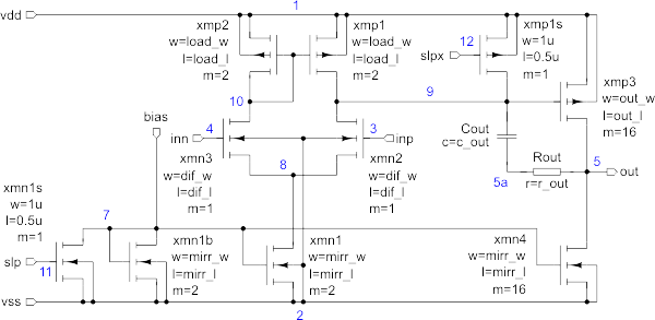
Opamp schematic (opamp.inc).

The opamp.inc file describes an opamp in form as a subcircuit.

* Simple opamp, 0.18u, 1.8V, SpiceOpus
.include 'mosmm.inc'

* Operating conditions - fixed
.param ibias=1.000000000000e-004 

* Design parameters - fixed
.param c_out=8.211596855053e-012
.param r_out=1.968986740568e+001

* inp inn out vdd vss bias slp slpx
.subckt amp 3 4 5 1 2 7 11 12
xmp1 9 10 1 1  submodp w={load_w} l={load_l} m=2
xmp2 10 10 1 1 submodp w={load_w} l={load_l} m=2
xmp1s 9 12 1 1 submodp w=1u        l=0.5u
xmp3 5 9 1 1   submodp w={out_w}   l={out_l}   m=16
xmn2 9 3 8 2   submodn w={dif_w}   l={dif_l} 
xmn3 10 4 8 2  submodn w={dif_w}   l={dif_l} 
xmn1s 7 11 2 2 submodn w=1u        l=0.5u
xmn1b 7 7 2 2  submodn w={mirr_w}  l={mirr_l}  m=2
xmn1 8 7 2 2   submodn w={mirr_w}  l={mirr_l}  m=2
xmn4 5 7 2 2   submodn w={mirr_w}  l={mirr_l}  m=16
cout 5a 9 c={c_out}
rout 5 5a r={r_out}
.ends

Any include or lib file that will be specified in PyOPUS must not be included here with .include or .lib. The same holds for all circuit parameters that will be controlled by PyOPUS. They must not be specified here with .param statements.

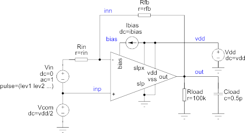
Opamp testbench circuit schematic (topdc.inc).

The topdc.inc file specifies a simple testbench circuit

* Test topology
x1 (inp inn out vdd 0 bias 0 vdd) amp
vdd (vdd 0) dc={vdd}
ibias (vdd bias) dc={ibias}
rfb (out inn) r={rfb}
rin (in inn) r={rin}
vcom (inp 0) dc={vdd/2}
vin (in inp) dc=0 acmag=1 pulse=({lev1} {lev2} {tstart} {tr} {tf} {pw})
rload (out 0) r=100k
cload (out 0) c=0.5p

The opamp is represented by the x1 subcircuit.

Note that none of the above listed .inc files has an .end directive. The .end directive will be added by PyOPUS when it joins the source files together and simulates the circuit by invoking SPICE OPUS.

The runme.py file is quite long. Let's explain it. The explanations are Python comments (#).

# Optimize with cost evaluator and iteration plotter

# Import PyOPUS components

# This one is for evaluating the circuit's performance, e.g. extracting things 
# like gain, bandwidth, etc. from responses generated by the simulator. 
from pyopus.evaluator.performance import PerformanceEvaluator

# This one constructs the cost function from circuit's perfomance. 
# parameterSetup is a convenience function that prepares upper and lower bounds 
# on parameters that are later passed to the constrained optimizer. 
from pyopus.evaluator.aggregate import *

# This one converts a parameter description dictionary to parameter value lists
from pyopus.evaluator.auxfunc import listParamDesc

# This is the top wrapper for selecting the optimization algorithm. 
from pyopus.optimizer import optimizerClass

# This is the plotting facility based on MatPlotLib and WxPython. It plots 
# the ciruit's response every time it gets invoked. 
from pyopus.visual.wxmplplotter import WxMplPlotter

# This one plots the circuit's response every time a candidate circuit is 
# evaluated by the optimizer. 
from pyopus.visual.plotter import IterationPlotter

# Need to protect the main program from being evaluated at import. 
# If not, we get an infinite loop when multiprocessing forks the gui thread. 
if __name__=='__main__':
	# This Python dictionary specifies the simulator(s) and the input files
	heads = {
		# An entry for the SPICE OPUS simulator
		'opus': {
			# Here we specify the entry uses SPICE OPUS
			'simulator': 'SpiceOpus', 
			# Additional parameters passed to the constructor of SpiceOpus 
			# simulator object instance (Python wrapper for SPICE OPUS)
			'settings': {
				'debug': 0
			}, 
			# Define circuit blocks used by PyOPUS when simulating the circuit
			'moddefs': {
				'def':     { 'file': 'opamp.inc' }, 
				'tb':      { 'file': 'topdc.inc' }, 
				'mos_tm': { 'file': 'cmos180n.lib', 'section': 'tm' }, 
				'mos_wp': { 'file': 'cmos180n.lib', 'section': 'wp' }, 
				'mos_ws': { 'file': 'cmos180n.lib', 'section': 'ws' }, 
				'mos_wo': { 'file': 'cmos180n.lib', 'section': 'wo' }, 
				'mos_wz': { 'file': 'cmos180n.lib', 'section': 'wz' }
			}, 
			# Simulator options (.options) common to all analyses run by this 
			# simulator wrapper instance
			'options': {
				'method': 'trap'
			}, 
			# Circuit parameters (.param) common to all analyses run by this 
			# simulator wrapper instance 
			'params': {
				'lev1': 0.0,
				'lev2': 0.5,
				'tstart': 1e-9, 
				'tr': 1e-9, 
				'tf': 1e-9, 
				'pw': 500e-9
			}
		}
	}
	
	# Python variables that are accessible in the var dictionary
	# We list here the MOS instances and their properties that need to be saved during analysis
	variables={
		'saveInst': [ 'xmn2', 'xmn3', 'xmn1' ], 
		'saveProp': [ 'vgs', 'vth', 'vds', 'vdsat' ]
	}

	# A dictionary specifying all analyses that need to be performed for 
	# evaluating this circuit
	analyses = {
		# Operating point analysis
		'op': {
			# Uses the �pus'head entry (i.e. simulates using SPICE OPUS)
			'head': 'opus', 
			# Uses the 'def' and the 'tb' circuit modules in this analysis 
			'modules': [ 'def', 'tb' ], 
			# Specify additional simulator options (.options) for this analysis 
			'options': {
				'method': 'gear'
			}, 
			# Specify additional circuit parameters (.param) for this analysis
			'params': {
				'rin': 1e6,
				'rfb': 1e6
			},
			# Save current through vdd. Save voltages at inp, inn, and out. 
			# Save instance output parameters vgs, vth, vds, and vdsat 
			# for core instance m0 inside xmn2, xmn3, and xmn1 which are part 
			# of x1. 
			'saves': [ 
				"i(['vdd'])", 
				"v(['inp', 'inn', 'out'])", 
				"p(ipath(var['saveInst'], 'x1', 'm0'), var['saveProp'])"
			],  
			# The actual command for running the analysis
			'command': "op()"
		}, 
		# DC analysis (sweeps input differential voltage)
		'dc': {
			'head': 'opus', 
			'modules': [ 'def', 'tb' ], 
			'options': {
				'method': 'gear'
			},
			'params': {
				'rin': 1e6,
				'rfb': 1e6
			},	
			'saves': [ ], 
			# This time the command is more complex
			# The arguments are: start, stop, sweep type, number of points, 
			#                    instance, and parameter
			'command': "dc(-2.0, 2.0, 'lin', 100, 'vin', 'dc')"
		}, 
		# Another DC analysis (sweeps input common mode voltage)
		'dccom': {
			'head': 'opus', 
			'modules': [ 'def', 'tb' ], 
			'options': {
				'method': 'gear'
			},
			'params': {
				'rin': 1e6,
				'rfb': 1e6
			},			
			'saves': [ 
				"v(['inp', 'inn', 'out'])", 
				"p(ipath(var['saveInst'], 'x1', 'm0'), var['saveProp'])"
			], 
			'command': "dc(0, param['vdd'], 'lin', 20, 'vcom', 'dc')"
		}
	}

	# This dictionary specifies the corners (operating conditions) in which 
	# the circuit's performance will be evaluated. 
	corners = {
		'nominal': {
			# In corner 'nominal' the mos_tm module is included which specifies
			# the typical NMOS and PMOS models from cmos180n.lib
			'modules': [ 'mos_tm' ], 
			# Specify circuit parameters (.param) for this corner. 
			# temperature is special and is interpreted by SpiceOpus wrapper 
			# as temp simulator option.
			'params': {
				'temperature': 25, 
				'vdd': 1.8, 
			}
		},
		'worst_power': {
			'modules': [ 'mos_wp' ], 
			'params': {
				'temperature': 100, 
				'vdd': 2.0, 
			}
		},
		'worst_speed': {
			'modules': [ 'mos_ws' ], 
			'params': {
				'temperature': 100, 
				'vdd': 1.8, 
			}
		}, 
		'worst_zero': {
			'modules': [ 'mos_wz' ], 
			'params': {
				'temperature': 100, 
				'vdd': 1.8, 
			}
		}, 
		'worst_one': {
			'modules': [ 'mos_wo' ], 
			'params': {
				'temperature': 100, 
				'vdd': 1.8, 
			}
		}
	}

	# Here we specify what we want to extract from simulation results
	# (performance measures)
	measures = {
		# Opamp supply current at operating point
		'isup': {
			# Gets extracted from 'op' analysis results
			'analysis': 'op', 
			# Evaluated across these corners
			'corners': [ 'nominal', 'worst_power', 'worst_speed' ], 
			# Extraction script (Python). The final result must be placed in 
			# the __result variable. 
			'script': "__result=-i('vdd')"
		}, 
		# Opamp otuput voltage at operating point
		'out_op': {
			'analysis': 'op', 
			'corners': [ 'nominal', 'worst_power', 'worst_speed' ], 
			'expression': "v('out')"
		},
		# Vgs overdrive (Vgs-Vth) for mn2, mn3, and mn1 at operating point
		'vgs_drv': {
			'analysis': 'op', 
			'corners': [ 'nominal', 'worst_power', 'worst_speed', 'worst_one', 'worst_zero' ], 
			'expression': """array(
				map(
					m.Poverdrive(p, 'vgs', p, 'vth'), 
					ipath(['xmn2', 'xmn3', 'xmn1'], 'x1', 'm0')
				)
			)""", 
			'vector': True
		}, 
		# Vds overdrive (Vds-Vdsat) for mn2, mn3, and mn1 at operating point
		'vds_drv': {
			'analysis': 'op', 
			'corners': [ 'nominal', 'worst_power', 'worst_speed', 'worst_one', 'worst_zero' ], 
			'expression': """array(
				map(
					m.Poverdrive(p, 'vds', p, 'vdsat'), 
					ipath(['xmn2', 'xmn3', 'xmn1'], 'x1', 'm0')
				)
			)""", 
			'vector': True
		}, 
		# Swing at gain (opamp output voltage span where fifferential gain is 
		# above 50% of maximal gain)
		'swing': {
			'analysis': 'dc', 
			'corners': [ 'nominal', 'worst_power', 'worst_speed', 'worst_one', 'worst_zero' ], 
			'expression': "m.DCswingAtGain(v('out'), v('inp', 'inn'), 0.5, 'out')"
		},
		# Gate area of current mirror transistors. No analysis is needed to 
		# evaluate this. 
		'mirr_area': {
			'analysis': None, 
			'corners': [ 'nominal' ], 
			'expression': (
				"param['mirr_w']*param['mirr_l']*(2+2+16)"
			)
		}, 
		# Input differential voltage values from 'dc' analysis (for plotting)
		'dcvin': {
			'analysis': 'dc', 
			'corners': [ 'nominal', 'worst_power', 'worst_speed', 'worst_one', 'worst_zero' ], 
			'expression': "v('inp', 'inn')",
			# Indicated the result is a vector. If we ommit this an exception 
			# is raised by PyOPUS at evaluation. 
			'vector': True
		},
		# Output voltage values from 'dc' analysis (for plotting)
		'dcvout': {
			'analysis': 'dc', 
			'corners': [ 'nominal', 'worst_power', 'worst_speed', 'worst_one', 'worst_zero' ], 
			'expression': "v('out')",
			'vector': True
		},
		# Input common mode voltage values from 'dccom' analysis (for plotting)
		'dccomvin': {
			'analysis': 'dccom', 
			'corners': [ 'nominal', 'worst_power', 'worst_speed', 'worst_one', 'worst_zero' ], 
			'expression': "v('inp')",
			'vector': True
		},
		# Output voltage values from 'dccom' analysis (for plotting)
		'dccomvout': {
			'analysis': 'dccom', 
			'corners': [ 'nominal', 'worst_power', 'worst_speed', 'worst_one', 'worst_zero' ], 
			'expression': "v('out')",
			'vector': True
		},
		# Vds-Vdsat (Vds overdrive) voltage values for mn1 from 'dccom' 
		# analysis (for plotting)
		'dccom_m1vdsvdsat': {
			'analysis': 'dccom', 
			'corners': [ 'nominal', 'worst_power', 'worst_speed', 'worst_one', 'worst_zero' ], 
			'expression': "p(ipath('xmn1', 'x1', 'm0'), 'vds')-p(ipath('xmn1', 'x1', 'm0'), 'vdsat')",
			'vector': True
		}
	}

	# Order in which circuit's performance measures are printed.
	# Note that we ommit all measures that will be plotted (we don't want to  
	# print a bunch of values from those long vectors). 
	outOrder = [ 
		'mirr_area', 'isup', 'out_op', 
		'vgs_drv', 'vds_drv', 
		'swing', 
	]
	
	# Circuit parameters (.param) subject to optimization (input parameters) 
	costInput = { 
		'mirr_w': {
			# Initial value
			'init': 7.456e-005, 
			# Lower bound
			'lo':	1e-6, 
			# Upper bound
			'hi':	95e-6, 
			# Step for discrete optimization algorithms. 
			# At present no such algorithm is avaliable. 
			'step':	0.01e-6
		},
		'mirr_l': {
			'init': 5.6e-007, 
			'lo':	0.18e-6, 
			'hi':	4e-6, 
			'step':	0.01e-6
		},
		'out_w': {
			'init': 4.801e-005, 
			'lo':	1e-6, 
			'hi':	95e-6, 
			'step':	0.01e-6
		},
		'out_l': {
			'init': 3.8e-007, 
			'lo':	0.18e-6, 
			'hi':	4e-6, 
			'step':	0.01e-6
		},
		'load_w': {
			'init': 3.486e-005, 
			'lo':	1e-6, 
			'hi':	95e-6, 
			'step':	0.01e-6
		},
		'load_l': {
			'init': 2.57e-006, 
			'lo':	0.18e-6, 
			'hi':	4e-6, 
			'step':	0.01e-6
		},
		'dif_w': {
			'init': 7.73e-006, 
			'lo':	1e-6, 
			'hi':	95e-6, 
			'step':	0.01e-6
		},
		'dif_l': {
			'init': 1.08e-006, 
			'lo':	0.18e-6, 
			'hi':	4e-6, 
			'step':	0.01e-6
		},
	}

	# Order in which input parameters are printed (sortes alphabetically)
	inOrder=costInput.keys()
	inOrder.sort()
	
	# This specifies how performance measures are processed in order to obtain 
	# the cost function (scalar) that is minimized by the optimization 
	# algorithm. 
	costDefinition = [
		{
			# Measurement name
			'measure': 'isup', 
			# This measurement should be below goal. Arguments to MNbelow() are 
			# goal, norm, and penalty that is applied when evaluation fails. 
			# Default norm is 1/10 of goal or 1 if goal is 0. 
			# Default failure penalization is 10000.0. 
			'norm': Nbelow(1e-3, 0.1e-3, 10000.0),	
			# This is the default cost contribution shape - 
			# linear2 with penalty weight 1 and tradeoff weight 0. 
			# Tradeoff weight 0 means that when the goal is reached further 
			# improvements to isup won't decrease the cost function value. 
			'shape': Slinear2(1.0,0.0), 
			# Corner reduction method (i.e. how to join the values calculated 
			# for individual corners into a single scalar cost contribution). 
			# here we say that we don't want to include this performance mesure 
			# in teh cost function. 
			'reduce': Rexcluded()					
		},
		{
			'measure': 'out_op',
			# Should be below 10
			'norm': Nbelow(10, 0.1e-3),
			'shape': Slinear2(1.0,0.0),
			# Do not include in cost function. 
			'reduce': Rexcluded()
		},
		{
			'measure': 'vgs_drv', 
			# Should be above 0.001. 
			'norm': Nabove(1e-3),, 					
			# Include only the worst corner's contribution in cost function. 
			# This is the default. 
			'reduce': Rworst()
		},
		{
			'measure': 'vds_drv', 
			# Should be above 0.001. 
			'norm': Nabove(1e-3)
		},
		{
			'measure': 'swing', 
			# Should be above 1.5
			'norm': Nabove(1.5), 
			# Tradeoff weight is 0.001 which means that the optimizer will try 
			# to improve this beyond the specified goal. 
			'shape': Slinear2(1.0,0.001), 
		},
		{
			'measure': 'mirr_area', 
			# Should be below 800 um^2
			'norm': Nbelow(800e-12, 100e-12), 
			# Tradeoff weight is 0.001 which means that the optimizer will try 
			# to improve this beyond the specified goal. 
			'shape': Slinear2(1.0,0.001)
		}
	]

	# Here we specify what will be plotted by the WxMplPlotter instance. 
	visualisation = {
			# Window list with axes
			'graphs': {
				# This window will display the DC sweep results (differential 
				# and common mode). 
				'dc': {
					# Window title
					'title': 'Amplifier DC response', 
					# Window shape (6x8 inches, 80dpi)
					'shape': { 'figsize': (6,8), 'dpi': 80 }, 
					# This specifies the axes (subplots) in inside the window 
					'axes': {
						# Axes for differential input voltage DC sweep
						'diff': {
							# Subdivide window in a grid with 2 vertical and 
							# 1 horizontal subplot. These axes represent the 
							# upper (first) subplot. This is same as in Matlab. 
							'subplot': (2,1,1), 
							# Extra options for the MatPlotLib 
							# Figure.add_subplot() method. 
							'options': {}, 
							# Grid type is rectangular (cartesian). 
							# This is the default. 
							# Also available: 'polar'
							'gridtype': 'rect', 		
							# Type of x-axis scale. 'linear' is the default. 
							'xscale': { 'type': 'linear' }, 
							# Type of x-axis scale. 'linear' is the default. 
							'yscale': { 'type': 'linear' }, 
							# x-axis scale limits. Default is autoscale. 
							'xlimits': (-50e-3, 50e-3), 
							# x-axis label
							'xlabel': 'Vdif=Vinp-Vinn [V]', 
							# y-axis label
							'ylabel': 'Vout [V]', 
							# Subplot title
							'title': '', 
							# Do we want a legend? Default is False. 
							'legend': False, 
							# Do we want to display a grid? 
							'grid': True, 
						}, 
						# Axes for common mode input voltage DC sweep
						'com': {
							# This is the lower (second) subplot. 
							'subplot': (2,1,2), 
							'options': {}, 
							'gridtype': 'rect', 
							'xscale': { 'type': 'linear' }, 
							'yscale': { 'type': 'linear' }, 
							'xlimits': (0.0, 2.0),
							'xlabel': 'Vcom=Vinp=Vinn [V]', 
							'ylabel': 'Vout [V]', 
							'title': '', 
							'legend': False, 
							'grid': True, 
						}
					}
				},
				# Another plot window for displaying the Vds overdrive voltage 
				# of mn1 (instance xmn1).  
				'm1vds': {
					'title': 'M1 Vds-Vdsat in common mode', 
					'shape': { 'figsize': (6,4), 'dpi': 80 }, 
					'axes': {
						# Only one axes in thios window. 
						'dc': {
							# This time we specify the relative position and 
							# size of the axes (x=0.12, y=0.12, w=0.76 h=0.76). 
							'rectangle': (0.12, 0.12, 0.76, 0.76), 
							'options': {}, 
							'gridtype': 'rect', 
							'xscale': { 'type': 'linear' }, 
							'yscale': { 'type': 'linear' }, 
							'xlimits': (0.0, 2.0), 
							'xlabel': 'Vcom=Vinp=Vinn [V]', 
							'ylabel': 'M1 Vds-Vdsat [V]', 
							'title': '', 
							'legend': False, 
							'grid': True, 
						}, 
					}
				}
			}, 
			# Here we define the trace style for the traces that will be 
			# plotted inside axes. The styles are applied in the same order 
			# as they are listed. Only those styles are applies that match the 
			# pattern specified by (graph, axes, corner, trace) name. The name 
			# can be a regular expression (see re Python module). 
			'styles': [ 
				# This one matches all plot windows (graphs), all axes, 
				# all corners and all traces. Everything will be plotted as red 
				# lines. 
				{
					'pattern': ('^.*', '^.*', '^.*', '^.*'), 
					# Style is specified as keyword arguments to the 
					# Axes.plot() method (see MatPlotLib docs). 
					'style': {
						'linestyle': '-',
						'color': (0.5,0,0)
					}
				}, 
				# This one matches all plot windows and all axes. Apllies only 
				# to traces generated for corners whose name starts with 'nom'. 
				# Matches all traces. Basically nominal traces will be plotted 
				# as green lines. 
				{
					'pattern': ('^.*', '^.*', '^nom.*', '^.*'),
					'style': {
						'linestyle': '-',
						'color': (0,0.5,0)
					}
				}
			], 
			# Trace list - what to plot and where 
			'traces': {
				# Defines the traces coming from differential input voltage 
				# sweep representing output vs input. 
				'dc': {
					# Plot them in the 'dc' graph (i.e. window)
					'graph': 'dc', 
					# on the 'diff' axes (upper subplot)
					'axes': 'diff', 
					# The x coordinates come from the 'dcvin' performance 
					# measure (remember that it is a vector). 
					'xresult': 'dcvin',
					# The y coordinates come from the 'dcvout' performance 
					# measure. 
					'yresult': 	'dcvout', 
					# Leaving this list empty or unspecified plots the trace 
					# across all evaluated corners. 
					'corners': [ ],	
					# Apply this style to the traces (solid line with 
					# dot markers). 
					'style': {	
						'linestyle': '-',
						'marker': '.', 
					}
				}, 
				# Defines the traces coming from common mode input voltage 
				# sweep representing output vs input. 
				'dccom': {
					# Plot in 'dc' window 
					'graph': 'dc', 
					# on the 'com' axes (lower subplot)
					'axes': 'com', 
					# The rest should be simple to understand. 
					'xresult': 'dccomvin',
					'yresult': 	'dccomvout', 
					'corners': [ ],	
					'style': {	
						'linestyle': '-',
						'marker': '.', 
					}
				},
				# Defines the traces coming from differential input voltage 
				# sweep representing output vs input. 
				'dc1': {
					# We didn't specify this window ('dccomb'). 
					# Nothing will be plotted. 
					'graph': 'dccomb', 
					'axes': 'dc', 
					'xresult': 'dcvin',
					'yresult': 	'dcvout', 
					# Plot only traces corresponding to the nominal corner. 
					'corners': [ 'nominal' ], 
					'style': {	
						'linestyle': '-',
						'marker': '.', 
					}
				}, 
				# Defines the traces coming from common mode input voltage 
				# sweep representing output vs input. 
				'dccom1': {
					# We didn't specify this window ('dccomb'). 
					# Nothing will be plotted. 
					'graph': 'dccomb', 
					'axes': 'dc', 
					'xresult': 'dccomvin',
					'yresult': 	'dccomvout', 
					'corners': [ 'nominal' ],	
					'style': {	
						'linestyle': '-',
						'marker': '.', 
					}
				},
				# Defines the traces coming from common mode input voltage 
				# sweep representing mn1 Vds ovedrive voltage vs input. 
				'm1_vds_vdsat': {
					# Plot in 'm1vds' window
					'graph': 'm1vds', 
					# on the 'dc' axes. 
					'axes': 'dc', 
					'xresult': 'dccomvin',
					'yresult': 	'dccom_m1vdsvdsat', 
					'corners': [ 'nominal' ],	
					'style': {	
						'linestyle': '-',
						'marker': '.', 
					}
				}
			}
		}

	# Now here is the program. 
	
	# Construct performance evaluator. 
	pe=PerformanceEvaluator(heads, analyses, measures, corners, variables=variables, debug=0)

	# Construct cost function evaluator (uses the performance evaluator 
	# for getting the circuit's performance). 
	ce=Aggregator(pe, costDefinition, inOrder, debug=0)

	# Extract initial value, lower and upper bound, and step for cost 
	# function's input parameters (parameters subject to optimization). 
	xlow=listParamDesc(costInput, inOrder, "lo")
	xhi=listParamDesc(costInput, inOrder, "hi")
	xinit=listParamDesc(costInput, inOrder, "init")
	
	# Construct a Hooke-Jeeves optimizer that will be used for optimizing 
	# the cost function (calculated by the ce cost evaluator instance). 
	# Specify parameter bounds. Limit number of iterations (candidate circuits) 
	# to 1000. 
	opt=optimizerClass("HookeJeeves")(ce, xlo=xlow, xhi=xhigh, maxiter=1000)

	# Set initial point. Accepts a Python list or 1-D Numpy array. 
	opt.reset(xinit)

	# Install reporter plugin into the optimizer. 
	# The plugin is obtained from the cost evaluator. 
	# It prints the cost function details every time cost is decreased. 
	opt.installPlugin(ce.getReporter())

	# Install stopper plugin into the optimizer. 
	# Stops optimization when all requirements are satisfied 
	# (all cost contributions are <=0). 
	# The plugin is obtained from the cost evaluator. 
	opt.installPlugin(ce.getStopWhenAllSatisfied())

	# Construct plotter that can plot the evaluation results. 
	# This uses the performanceevaluator to get the results and visualizes them 
	# according to the setting specified by the 'visualisation' dictionary. 
	plotter=WxMplPlotter(visualisation, pe)

	# Create and install iteration plotter plugin into teh optimizer. 
	# This wil plot the circuit's performance using plotter every time the 
	# best-yet cost function value is decreased. 
	opt.installPlugin(IterationPlotter(plotter))

	# Run optimization 
	opt.run()

	# Optimization results can be collected from the optimizer object. 
	# Parameter values of best circuit. 
	xresult=opt.x
	# Iteration number where the best circuit was obtained. 
	iterresult=opt.bestIter
	
	# Last circuit evaluation may not be the one where the best circuit was 
	# found. Therefore reevaluate the best circuit so performance evaluator 
	# and cost evaluator will hold the best circuit's performance measures 
	# and cost function value. 
	cf=ce(xresult)
		
	# Print results. 
	print(
		"\n\nFinal cost: "+str(cf)+
		", found in iter "+str(iterresult)+
		", total "+str(opt.niter)+" iteration(s)"
	)
	
	# Print final cost and iteration when it was found
	print("\n\nFinal cost: "+str(cf)+", found in iter "+str(iterresult)+", total "+str(opt.niter)+" iteration(s)")
	
	# Print parameter values of the best circuit stored in the cost evaluator. 
	print(ce.formatParameters())
	
	# Print cost evaluator's details of the best circuit's cost function value 
	# stored in the cost evaluator. 
	# This is the same sort of output as the cost reporter printed at every 
	# cost function improvement while the optimizer was running. 
	print(ce.formatResults(nMeasureName=10, nCornerName=15))
	
	# Print best circuit's performance measures stored in performance evaluator. 
	print("Performance in corners")
	print(pe.formatResults(outOrder, nMeasureName=10, nCornerName=15))

	# Remove intermediate files and shut down all simulators used by the 
	# performance evaluator. 
	pe.finalize()

You can run the example by typing

python runme.py

in the terminal window (cmd.exe under Windows or any kind of xterm under Linux).

If the Python interpreter is not in the system PATH you must specify the full path to the Python executable. The cost function value will be printed for every iteration and the details will be printed every time a better circuit is found.

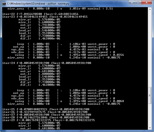
Output of the quickstart example in the terminal window.

Every time a better circuit is found (the best-yet cost function value decreses) the circuit's performance is plotted in two windows. When the optimization is finished (in this case when the stopper plugin stops the optimizer) the best circuit is re-evaluated and its performance in printed in the terminal window.

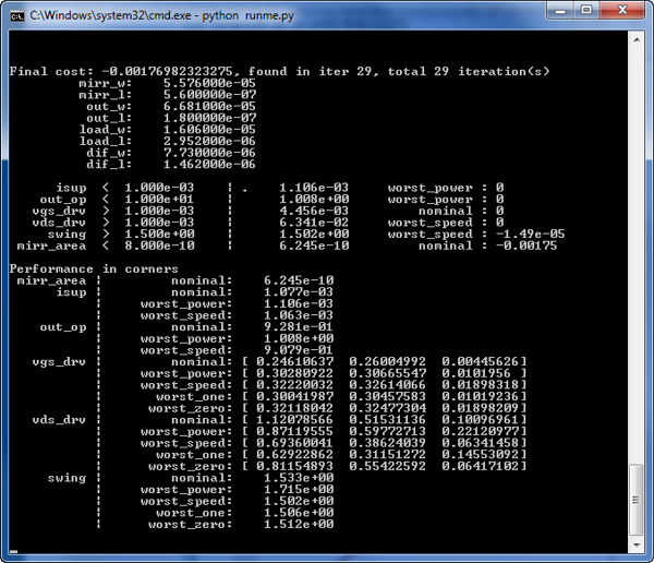
The performance of the best circuit that was found by the optimizer.

Also the performance of the final circuit is plotted in the same windows as the performance of the best-yet circuit was plotted during optimization.

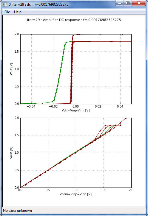
The dc plot window of the quickstart example (final result). Upper subplot is the differential input voltage sweep while the bottom window is the common mode input voltage sweep.

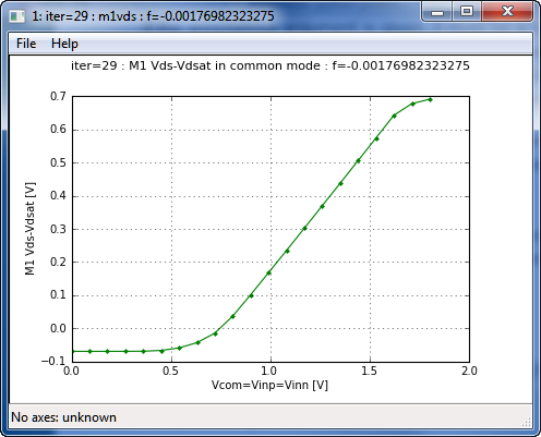
The m1vds plot window (final result) displaying the dependence of Vds overdrive voltage for mn1 (instance xmn1) with respect to the input common mode voltage.

To finish the demo, close the GUI control window.

The GUI control window.

3. Learning more about PyOPUS

You can start with the examples in the /demo subfolder of PyOPUS sources. Some demos are organzied as tutorials. Follow them in the same order as they are enumerated. A very useful resource is also the manual which was generated from docstrings in PyOPUS modules using Sphinx. Everything you see in the manual is also available through online Python help.