10.4.5. Plotting simulation results
This demo shows how to use the pyopus.visual.wxmplplotter.WxMplPlotter
class for plotting the simulation results. Read the Using the performance evaluator
chapter to learn more about the pyopus.evaluator.performance.PerformanceEvaluator class.
The problem definition in the main file runme.py in folder demo/evaluation/03-plotter/ is identical to the one in chapter Using the performance evaluator. Only the differences are given in this document.
First we must import the plotter and the MatPlotLib wrapper.
from pyopus.plotter.evalplotter import EvalPlotter
import pyopus.plotter as plt
We add a common mode DC sweep to the analyses (dccom).
	analyses = {
		'op': {
			'head': 'opus',
			'modules': [ 'def', 'tb' ],
			'options': {
				'method': 'gear'
			},
			'params': {
				'rin': 1e6,
				'rfb': 1e6
			},
			'saves': [
				"i(['vdd'])",
				"v(['inp', 'inn', 'out'])",
				"p(ipath(saveInst, 'x1', 'm0'), saveProp)"
			],
			'command': "op()"
		},
		'dc': {
			'head': 'opus',
			'modules': [ 'def', 'tb' ],
			'options': {
				'method': 'gear'
			},
			'params': {
				'rin': 1e6,
				'rfb': 1e6
			},
			'saves': [ ],
			'command': "dc(-2.0, 2.0, 'lin', 100, 'vin', 'dc')"
		},
		'dccom': {
			'head': 'opus',
			'modules': [ 'def', 'tb' ],
			'options': {
				'method': 'gear'
			},
			'params': {
				'rin': 1e6,
				'rfb': 1e6
			},
			'saves': [
				"v(['inp', 'inn', 'out'])",
				"p(ipath(saveInst, 'x1', 'm0'), saveProp)"
			],
			'command': "dc(0, param['vdd'], 'lin', 20, 'vcom', 'dc')"
		}
	}
Everything we want to plot must be collected by the evaluator. Therefore we add some mesurements that result in vectors from which we draw the x-y data for the plots (measures dcvin, dcvout, dccomvin, dccomvout, and dccom_m1vdsvdsat).
	measures = {
		# Supply current
		'isup': {
			'analysis': 'op',
			'corners': [ 'nominal', 'worst_power', 'worst_speed' ],
			'expression': "isup=-i('vdd')"
		},
		# Output voltage at zero input voltage
		'out_op': {
			'analysis': 'op',
			'corners': [ 'nominal', 'worst_power', 'worst_speed' ],
			'expression': "v('out')"
		},
		# Vgs overdrive (Vgs-Vth) for mn2, mn3, and mn1.
		'vgs_drv': {
			'analysis': 'op',
			'corners': [ 'nominal', 'worst_power', 'worst_speed', 'worst_one', 'worst_zero' ],
			'expression': "array(list(map(m.Poverdrive(p, 'vgs', p, 'vth'), ipath(saveInst, 'x1', 'm0'))))",
			'vector': True
		},
		# Vds overdrive (Vds-Vdsat) for mn2, mn3, and mn1.
		'vds_drv': {
			'analysis': 'op',
			'corners': [ 'nominal', 'worst_power', 'worst_speed', 'worst_one', 'worst_zero' ],
			'expression': "array(list(map(m.Poverdrive(p, 'vds', p, 'vdsat'), ipath(saveInst, 'x1', 'm0'))))",
			'vector': True
		},
		# DC swing where differential gain is above 50% of maximal gain
		'swing': {
			'analysis': 'dc',
			'corners': [ 'nominal', 'worst_power', 'worst_speed', 'worst_one', 'worst_zero' ],
			'expression': "m.DCswingAtGain(v('out'), v('inp', 'inn'), 0.5, 'out')"
		},
		# Surface area occupied by the current mirrors
		'mirr_area': {
			'analysis': None,
			'corners': [ 'nominal' ],
			'expression': (
				"param['mirr_w']*param['mirr_l']*(2+2+16)"
			)
		},
		# Input differential voltage from dc analysis (vector)
		'dcvin': {
			'analysis': 'dc',
			'corners': [ 'nominal', 'worst_power', 'worst_speed', 'worst_one', 'worst_zero' ],
			'expression': "v('inp', 'inn')",
			'vector': True
		},
		# Output voltage from dc analysis (vector)
		'dcvout': {
			'analysis': 'dc',
			'corners': [ 'nominal', 'worst_power', 'worst_speed', 'worst_one', 'worst_zero' ],
			'expression': "v('out')",
			'vector': True
		},
		# Input common mode voltage from dccom analysis (vector)
		'dccomvin': {
			'analysis': 'dccom',
			'corners': [ 'nominal', 'worst_power', 'worst_speed', 'worst_one', 'worst_zero' ],
			'expression': "v('inp')",
			'vector': True
		},
		# Output voltage from dccom analysis (vector)
		'dccomvout': {
			'analysis': 'dccom',
			'corners': [ 'nominal', 'worst_power', 'worst_speed', 'worst_one', 'worst_zero' ],
			'expression': "v('out')",
			'vector': True
		},
		# Vds overdrive for xmn1 from dccom analysis (vector)
		'dccom_m1vdsvdsat': {
			'analysis': 'dccom',
			'corners': [ 'nominal', 'worst_power', 'worst_speed', 'worst_one', 'worst_zero' ],
			'expression': "p(ipath('xmn1', 'x1', 'm0'), 'vds')-p(ipath('xmn1', 'x1', 'm0'), 'vdsat')",
			'vector': True
		},
	}
Now we define the plots for the plotter.
visualisation = {
# Window list with axes for every window
# Most of the options are arguments to MatPlotLib API calls
# Every plot window has its unique name by which we refer to it
'graphs': {
# One window for the DC response
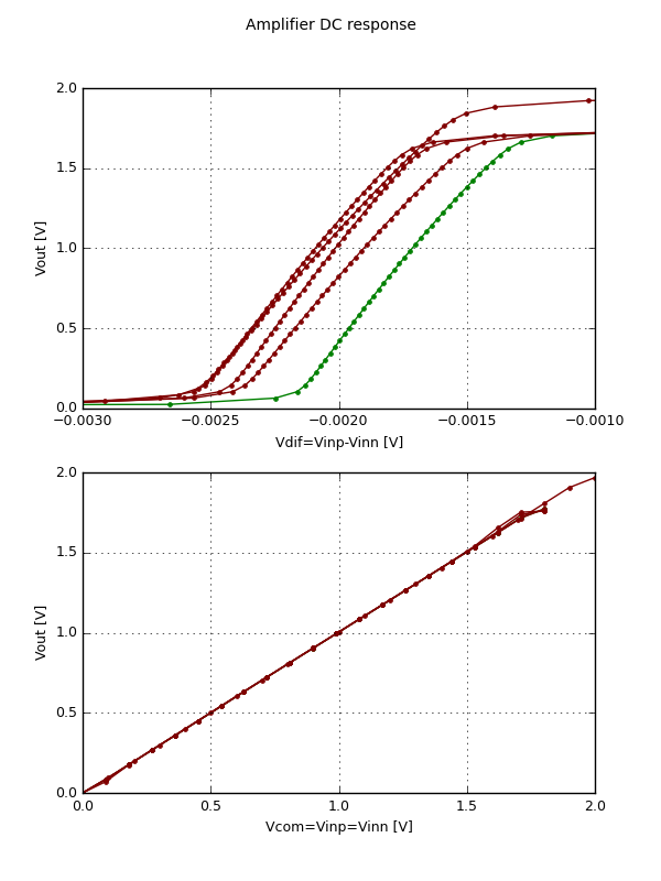
'dc': {
'title': 'Amplifier DC response',
'shape': { 'figsize': (6,8), 'dpi': 80 },
# Define the axes
# Every axes have a unique name by which we refer to them
'axes': {
# The first vertical subplot displays the differential response
'diff': {
# Argument to the add_subplot API call
'subplot': (2,1,1),
# Extra options
'options': {},
# Can be rect (default) or polar, xscale and yscale have no meaning when grid is polar
'gridtype': 'rect',
# linear by default, can also be log
'xscale': { 'type': 'linear' },
'yscale': { 'type': 'linear' },
'xlimits': (-3e-3, -1e-3),
'xlabel': 'Vdif=Vinp-Vinn [V]',
'ylabel': 'Vout [V]',
'title': '',
'legend': False,
'grid': True,
},
# The second vertical subplot displays the common mode response
'com': {
'subplot': (2,1,2),
'options': {},
'gridtype': 'rect',
'xscale': { 'type': 'linear' },
'yscale': { 'type': 'linear' },
'xlimits': (0.0, 2.0),
'xlabel': 'Vcom=Vinp=Vinn [V]',
'ylabel': 'Vout [V]',
'title': '',
'legend': False,
'grid': True,
}
}
},
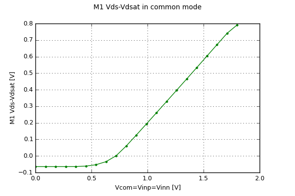
# Another window for the M1 Vds overdrive in common mode
'm1vds': {
'title': 'M1 Vds-Vdsat in common mode',
'shape': { 'figsize': (6,4), 'dpi': 80 },
'axes': {
'dc': {
# This time we define add_axes API call
'rectangle': (0.12, 0.12, 0.76, 0.76),
'options': {},
'gridtype': 'rect', # rect (default) or polar, xscale and yscale have no meaning when grid is polar
'xscale': { 'type': 'linear' }, # linear by default
'yscale': { 'type': 'linear' }, # linear by default
'xlimits': (0.0, 2.0),
'xlabel': 'Vcom=Vinp=Vinn [V]',
'ylabel': 'M1 Vds-Vdsat [V]',
'title': '',
'legend': False,
'grid': True,
},
}
}
},
# Here we define the trace styles. If pattern mathces a combination
# of (graph, axes, corner, trace) name the style is applied. If
# multiple patterns match one trace the style is the union of matched
# styles where matched entries that appear later in this list override
# those that appear earlier.
# The patterns are given in the format used by the :mod:`re` Python module.
'styles': [
{
# A default style (red, solid line)
'pattern': ('^.*', '^.*', '^.*', '^.*'),
'style': {
'linestyle': '-',
'color': (0.5,0,0)
}
},
{
# A style for traces representing the response in the nominal corner
'pattern': ('^.*', '^.*', '^nom.*', '^.*'),
'style': {
'linestyle': '-',
'color': (0,0.5,0)
}
}
],
# List of traces. Every trace has a unique name.
'traces': {
# Differential DC response in all corners
'dc': {
# Window an axes where the trace will be plotted
'graph': 'dc',
'axes': 'diff',
# Result vector used for x-axis data
'xresult': 'dcvin',
# Result vector used for y-axis data
'yresult': 'dcvout',
# Corners for which the trace will be plotted
# If not specified or empty, all corners where xresult is evaluated are plotted
'corners': [ ],
# Here we can override the style matched by style patterns
'style': {
'linestyle': '-',
'marker': '.',
}
},
# Common mode DC response in all corners
'dccom': {
'graph': 'dc',
'axes': 'com',
'xresult': 'dccomvin',
'yresult': 'dccomvout',
'corners': [ ],
'style': {
'linestyle': '-',
'marker': '.',
}
},
# Vds overdrive for M1 in common mode, nominal corner only
'm1_vds_vdsat': {
'graph': 'm1vds',
'axes': 'dc',
'xresult': 'dccomvin',
'yresult': 'dccom_m1vdsvdsat',
'corners': [ 'nominal' ],
'style': {
'linestyle': '-',
'marker': '.',
}
}
}
}
Finally we put it all together in the main program.
	# Construct performane evaluator
	pe=PerformanceEvaluator(heads, analyses, measures, corners, variables=variables, debug=0)

	# Construct plotter
	plotter=EvalPlotter(visualisation, pe, debug=1)

	# Evaluate performance
	results=pe(inParams)

	# Plot
	plotter()

	# Cleanup intermediate files
	pe.finalize()

	# Wait for windows to close
	# If we don't do this the program crashes immediately after the windows appear
	plt.join()