4.11. pyopus.optimizer.de — Box constrained differential evolution optimizer

Box constrained differential evolution global optimizer (PyOPUS subsystem name: DEOPT)

Published first in [de].

[de]	Storn R., Price K.: Differential evolution - a simple and efficient heuristic for global optimization over continuous spaces. Journal of Global Optimization vol. 11, pp. 341–359, 1997.

class pyopus.optimizer.de.DifferentialEvolution(function, xlo, xhi, debug=0, fstop=None, maxiter=None, maxSlaves=None, minSlaves=0, maxGen=None, spawnerLevel=1, populationSize=100, w=0.5, pc=0.3, seed=0)

Box constrained differential evolution global optimizer class

If debug is above 0, debugging messages are printed.

The lower and upper bound (xlo and xhi) must both be finite.

maxGen is the maximal number of generations. It sets an upper bound on the number of iterations to be the greater of the following two values: maxiter and .

populationSize is the number of inidividuals (points) in the population.

w is the differential weight between 0 and 2.

pc is the crossover probability between 0 and 1.

seed is the random number generator seed. Setting it to None uses the builtin default seed.

If spawnerLevel is not greater than 1, evaluations are distributed across available computing nodes (that is unless task distribution takes place at a higher level).

Infinite bounds are allowed. This means that the algorithm behaves as an unconstrained algorithm if lower bounds are and upper bounds are . In this case the initial population must be defined with the reset() method.

See the BoxConstrainedOptimizer for more information.

check()

Checks the optimization algorithm’s settings and raises an exception if something is wrong.

generatePoint(i)

Generates a new point through mutation and crossover.

initialPopulation()

Constructs and returns the initial population.

Fails if any bound is infinite.

reset(x0=None)

Puts the optimizer in its initial state.

x is eiter the initial point (which must be within bounds and is ignored) or the initial population in the form of a 2-dimensional array or list where the first index is the population member index while the second index is the component index. The initial population must lie within bounds xlo and xhi and have populationSize members.

If x is None the initial population is generated automatically. In this case xlo and xhi determine the dimension of the problem. See the initialPopulation() method.

run()

Run the algorithm.

Example file de.py in folder demo/optimizer/

Read Using MPI with PyOPUS if you want to run the example in parallel.

# Optimize SchwefelA function with differential evolution
# Collect cost function and plot progress
# Run the example with mpirun/mpiexec to use parallel processing

from pyopus.optimizer.de import DifferentialEvolution
from pyopus.problems import glbc
from pyopus.optimizer.base import Reporter, CostCollector, RandomDelay
import pyopus.plotter as pyopl
from numpy import array, zeros, arange
from numpy.random import seed
from pyopus.parallel.cooperative import cOS
from pyopus.parallel.mpi import MPI


if __name__=='__main__':
	cOS.setVM(MPI())
	
	ndim=30
	popSize=50
	
	prob=glbc.SchwefelA(n=ndim)
	slowProb=RandomDelay(prob, [0.001, 0.010])
	
	opt=DifferentialEvolution(
		slowProb, prob.xl, prob.xh, debug=0, 
		maxGen=150, populationSize=popSize, w=0.5, pc=0.3, seed=None
	)
	cc=CostCollector()
	opt.installPlugin(cc)
	opt.installPlugin(Reporter(onIterStep=1000))
	opt.reset()
	opt.run()
	cc.finalize()
	
	pyopl.init()
	pyopl.close()
	f1=pyopl.figure()
	pyopl.lock(True)
	if pyopl.alive(f1):
		ax=f1.add_subplot(1,1,1)
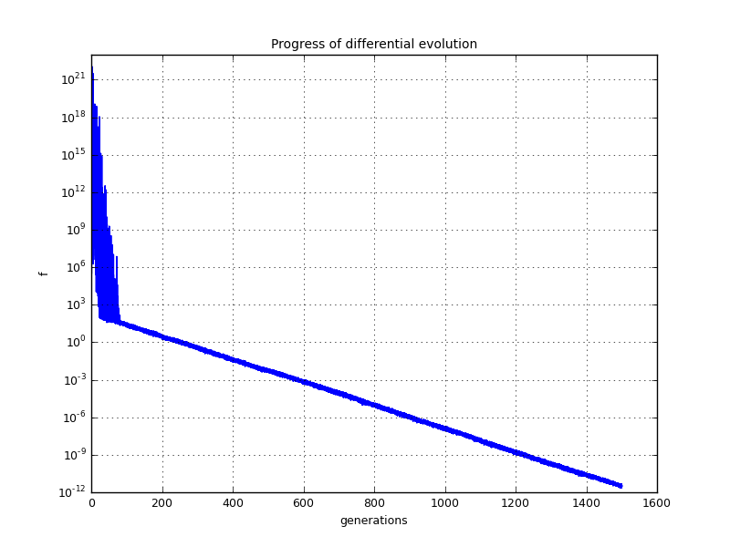
		ax.semilogy(arange(len(cc.fval))/popSize, cc.fval)
		ax.set_xlabel('generations')
		ax.set_ylabel('f')
		ax.set_title('Progress of differential evolution')
		ax.grid()
		pyopl.draw(f1)
	pyopl.lock(False)
	
	print("x=%s f=%e" % (str(opt.x), opt.f))
	
	pyopl.join()
	
	cOS.finalize()