11.4.3. Visualization of saved waveforms
Just like we can evaluate various performance measures from stored waveform we can also plot these waveforms. First, select a result node that contains stored waveforms in the result nodes tree. Under “Plots (post)” in the postprocessing tree you can define various plots based on the stored waveforms.
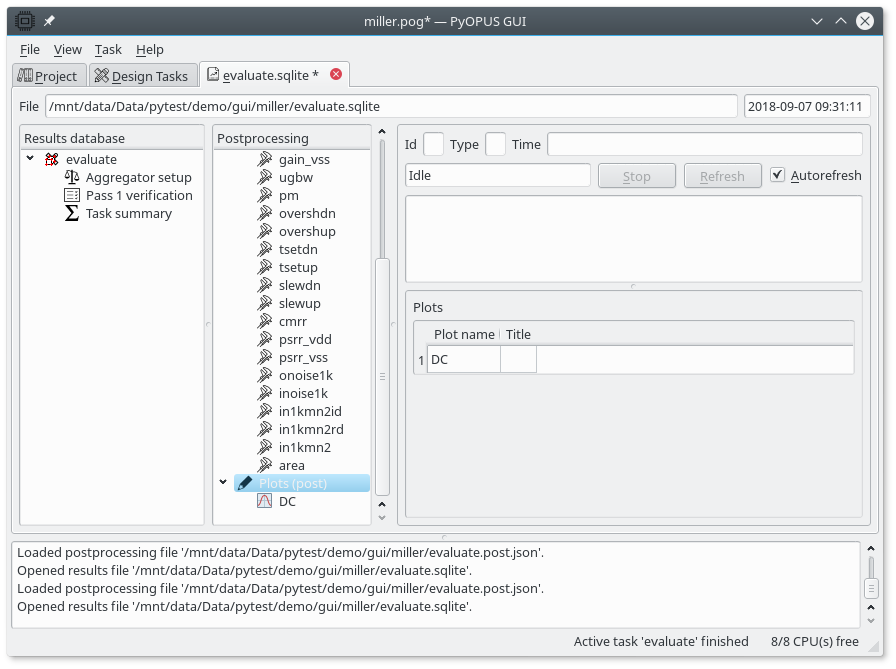
GUI displaying the summary of all defined plots.
The display area in the rightmost part of the results tab is divied in three parts. The top left part displays the plot, the top right part displays the messages generated during plot evaluation, and the bottom part is an editor for defining the properties of plots. The interface is similar to that used for defining and evaluating performance measures.
Every plot is divided in subplots also referred to as axes. Axes are organized in a rectangular grid. The coordinates of the top left cell in this grid are (0,0). The coordinates of the bottom right cell are (m-1,n-1) where m and n denote the number of cells in a column and row, respectively. Axes can span multple cells horizontally and vertically. For axes that occupy the whole plot area the horizonal and the vertical position are both 0, while the horizontal and vertical span are both 1. The philosophy is similar to the one used in Matlab for defining subplots.
To dubdivide the plot area in two axes positioned one above the other the top axes have origin (0,0) and span (1,1), while the bottom axes have origin (0,1) and span (1,1).
Now let us create a plot divided in two axes. Top axesdisplay the DC characteristic of the Miller opamp, while the bottom axes display the differential gain vs. the output voltage. A new plto can be created as a sub item under the “Plots (post)” tree item in the Postprocessing tree or it can be added as a new entry in the table summarizing all plots. This table is displayed if you select the “Plots (post)” tree item. The plot name must be a valid identifier. We choose “DC” as the plot name. The plot title is currently not displayed. It can be used for entering a short comment.
Axes are defined by adding subitems to the plot item in the Postprocessing tree. We create two subitems names “Response” and “Gain”. When any of them is selected its properties are listed in the editor on the bottom of the display area. The top left part of the display area will display the selected axes and all traces defined for the selected axes. The following properties can be set for axes.
Name - must be a valid identifier
Title - the title to display above the axes
X label - the label for the x-axis
Y label - the label for the y-axis
Plot type - can be Linear, Semi logarithmic (x), Semi logarithmic (y), or Logarithmic
Aspect ratio can be locked to 1:1 so that circles are drawn as circles and not as ellipses
Horizontal and vertical position and span defining the part of the plot the axes will occupy
Lower and upper limit for x and y axis for specifying the plot range. If the range is not specified autoscaling is used.
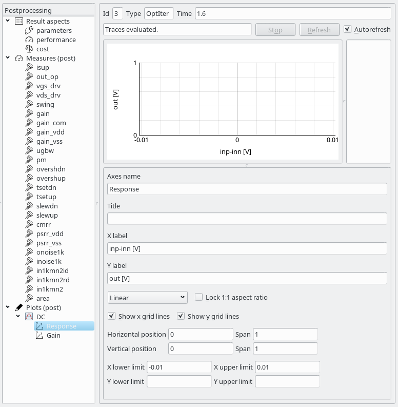
Setting up the DC response axes.
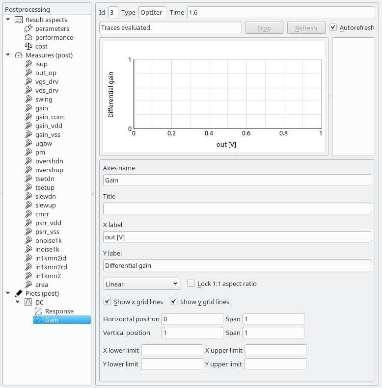
Setting up the DC gain axes.
Under every defined axes you can add one or more traces to display. A trace is added as a subitem of the axes item in the Postprocessing tree. When a trace is selected it is displayed in the top left part of the display. For every trace you can specify
Trace name - must be a valid indentifier.
Required analyses - a list of analyses that produced the waveforms from which the x and the y values for plotting the trace will be computed.
Expression for computing the y values
Optional expression for scale. If only one analysis is listed in the required analyses table and no scale expression is defined the default scale of the listed analysis is used.
When traces are defined that use the results of only one analysis the simulation results can be accessed with
<result access function>(<arguments>)
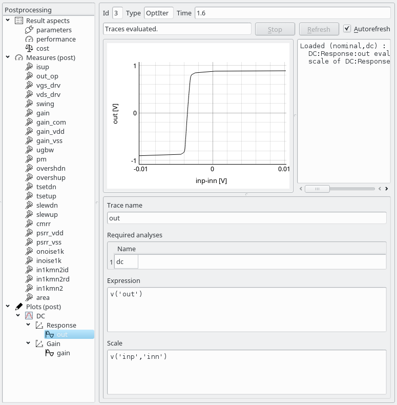
Setting up the DC response trace names “out”.
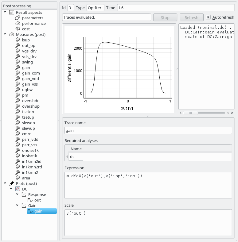
Setting up the DC gain trace named “gain”.
By moving the cursor over the plot a crosshair is displayed and its coordinates are printed. To identify a trace, slick on it. Its name will and the corner in which the circuit was simulated will be displayed.
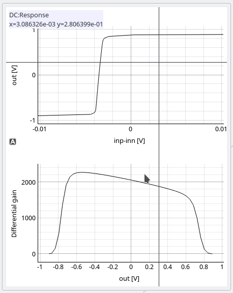
Crosshair and its position displayed for the top plot.
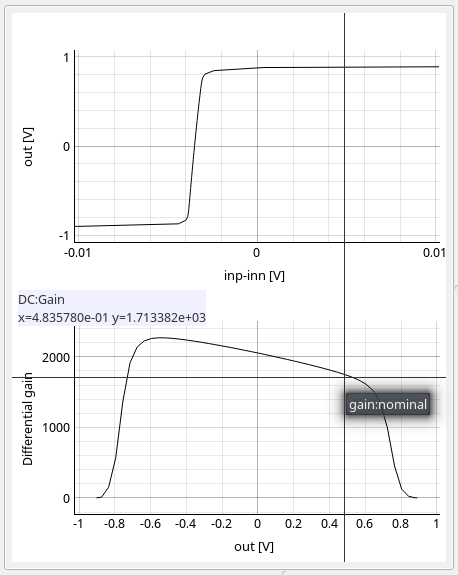
Identifying a trace in the bottom plot by clicking on it.
The displayed plot is updated every time a setting that affects it is changed if the “Autorefresh” checkbox is checked in the top right part of the display. During refresh the consistency of the plot setup is checked and errors are printed to the top right part of the display. Errors that occur during expression evaluation are also printed. The messages can be used for debugging the expressions for x and y values of a trace in the same manner as they were used in the previous section for debugging performance measures.
If a plot node is selected in the Postprocessing tree the corresponding plot with all of its axes is displayed.
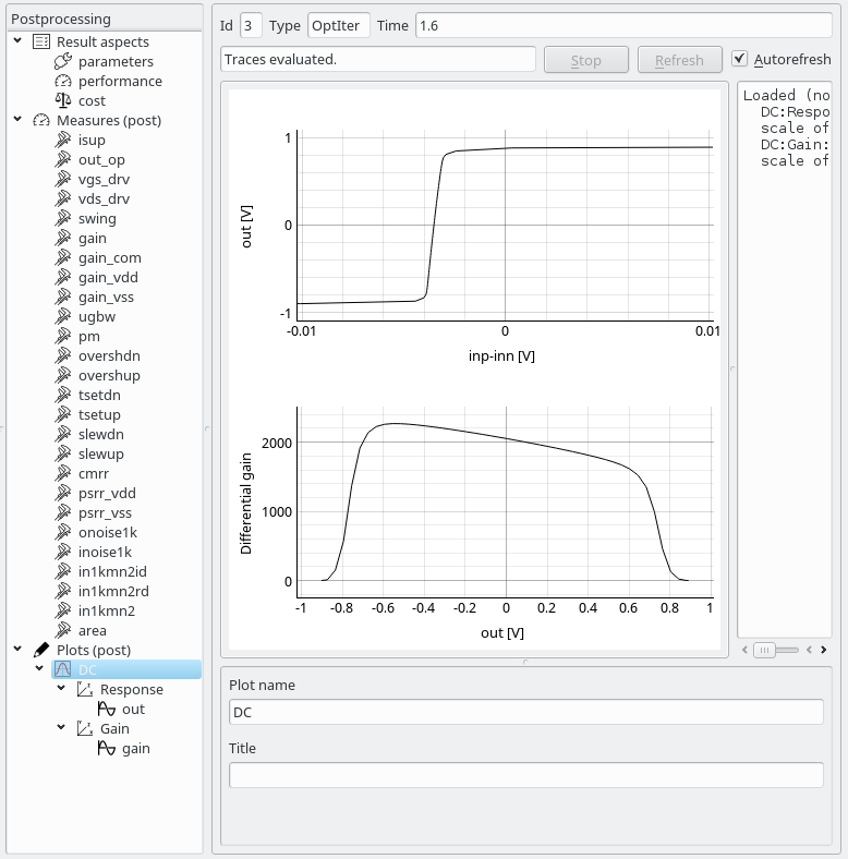
Viewing the complete DC plot.
Traces can be generated from the results of multiple analyses. If you want to plot the frequency response of CMRR for an opamp you will need the results of the AC analysis where differential excitation was applied and the results of the AC analysis where common mode excitation was applied. Both analyses must be performend on the same frequency scale so that points in the result vectors of both analysis correspond to same frequency points.
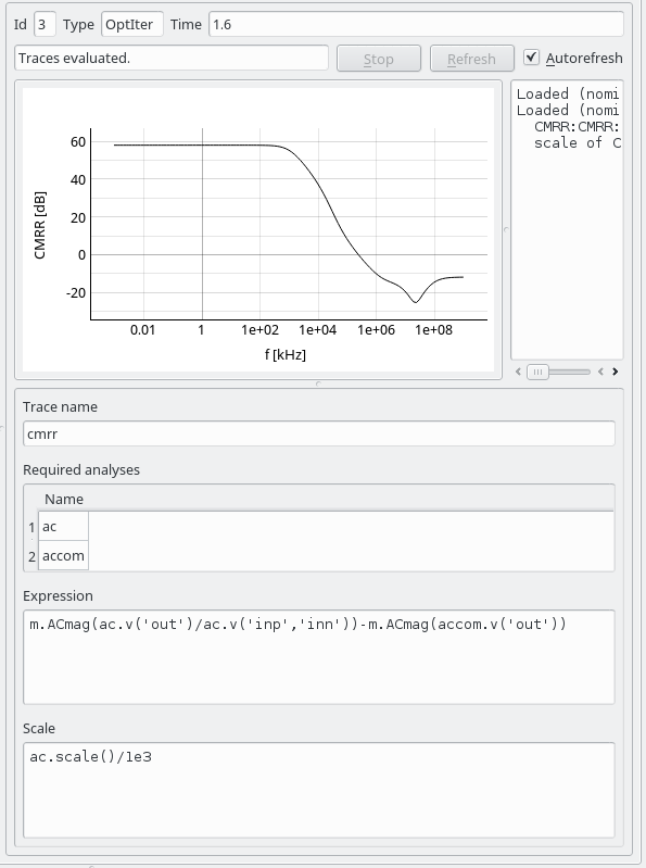
Setting up a trace for displaying the CMRR of an amplifier.
The CMRR trace depends on two analyses: ac and accom. Therefore
expressions that define the x and y axis values must now refer to the
simulation results as
<analysis name>.<result access function>(<arguments>)