5.10. pyopus.problems.cutermgr — CUTEr problem manager

CUTEr problem manager

Currently works only under Linux.

CUTEr is a collection of problems and a systef for interfacing to these problems. Every problem is described in a .sif file. This file is converted to FORTRAN code (evaluators) that evaluate the function’s terms and their derivatives. CUTEr provides fortran subroutines (CUTEr tools) that call evaluators and return things like the function’s value or the value of the function’s gradient at a given point, etc. CUTEr tools are available in a static library libcuter.a.

Every CUTEr problem is first compiled with a tool named sifdecode that produces the evaluators in FORTRAN. The evaluators are compiled and linked with the CUTEr tools and the Python interface to produce a loadable binary module for Python. The evaluators must be compiled with the same compiler as CUTEr tools. The loadable Python module is stored in a cache so that it does not have to be recompiled every time one wants to use the CUTEr problem.

Installing CUTEr

Before you use this module, you must build sifdecode and the CUTEr tools library.

Unpack the SIF decoder, build it by running install_sifdec (answers to the first five questions should be: PC, Linux, gfortran, double precision, large). Set the SIFDEC enavironmental variable so that it contains teh path to the folder where you unpacked the sifdecode source (where install_sifdec is located). After sifdecode is built a subfolder named SifDec.large.pc.lnx.gfo is created in $SIFDEC. Set the MYSIFDEC environmental variable so that it contains the path to this folder. Add $MYSIFDEC/bin to PATH so sifdecode will be accessible from anywhere. Also add $SIFDEC/common/man to the MANPATH environmental variable.

Unpack CUTEr. The tools library (libcuter.a) must be built with -fPIC (as position independent code). To achieve this, the file config/linux.cf in CUTEr installation must be edited and the -fPIC option added to lines that begin with:

#define FortranFlags ...
#define CFlags ...

Build the CUTEr library by running install_cuter (answers to the first five questions should be: PC, Linux, gfortran, GNU gcc, double precision, large). Set the CUTER environmental variable so that it contains the path to the folder where you unpacked CUTEr (the one where install_cuter is located). After CUTEr is compiled (i.e. libcuter.a is built) a subfolder named CUTEr.large.pc.lnx.gfo is created. Set the MYCUTER environmental variable so that it contains the path to this folder. Add $CUTER/common/man to MANPATH $CUTER/common/include to C_INCLUDE_PATH, $MYCUTER/double/lib to LIBPATH, and $MYCUTER/bin to PATH.

On 64-bit systems use the standard version of CUTEr (not the 64-bit one).

Download SIF files describing the available problems from http://www.cuter.rl.ac.uk/ and create a SIF repository (create a directory, unpack the problems, and set the MASTSIF environmental variable to point to the directory holding the SIF files).

The Python interface to CUTEr

Create a folder for the CUTEr cache. Set the PYCUTER_CACHE environmental variable to contain the path to the cache folder. Add $PYCUTER_CACHE to the PYTHONPATH envorinmental variable. The last step will make sure you can access the cached problems from Python.

If PYCUTER_CACHE is not set the current directory (.) is used for caching. Problems are cached in $PYCUTER_CACHE/pycuter.

The interface depends on gfortran and lapack. Make sure they are installed.

Once a problem is built only the following files in $PYCUTER_CACHE/pycuter/PROBLEM_NAME are needed for the problem to work:

• _pycuteritf.so – CUTEr problem interface module
• __init__.py – module initialization and wrappers
• OUTSDIF.d – problem information

A cached problem can be imported with from pycuter import PROBLEM_NAME. One can also use importProblem() which returns a reference to the problem module.

Available functions

• clearCache() – remove Python interface to problem from cache
• prepareProblem() – decode problem and build Python interface
• importProblem() – import problem interface module from cache (prepareProblem must be called first)
• isCached() – returns True if a problem is in cache

CUTEr problem structure

CUTEr provides constrained and unconstrained test problems. The objective function is a map from Rn to R:

where is a real scalar (member of ) and is a n-dimensional real vector (member of ). The i-th component of is denoted by and is also referred to as the i-th problem variable. Problem variables can be continuous (take any value from ), integer (take only integer values) or boolean (only 0 and 1 are allowed as variable’s value).

The optimization problem can be subject to simple bounds of the form

where and denote the lower and the upper bound on the i-th component of vector x. If there is no lower (or upper) bound on CUTEr reports (or ).

Beside simple bounds on problem variables some CUTEr problems also have more sophisticated constraints of the form

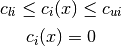
where is the i-th constraint function. The former is an inequality constraint while the latter is an equality constraint. CUTEr problems have generally m such constraints. In and the values -1e20 and 1e20 stand for and . For equality constraints and are both equal to 0. All constraint functions are joined in a single vector-valued function (map from to ) named .

CUTEr can order the constraints in such manner that equality constraints appear before inequality constraints. It is also possible to place linear constraints before nonlinear constraints. This of course reorders the components of c(x). Similarly variables (components of x) can also be reordered in such manner that nonlinear variables appear before linear ones.

The Lagrangian function, the Jacobian matrix, and the Hessian matrix

The Lagrangian function is defined as

Vector v is m-dimensional. Its components are the Lagrange multipliers.

The Jacobian matrix () is the matrix of constraint gradients. One row corresponds to one constraint function . The matrix has n columns. The element in the i-th row and j-th column is the derivative of the i-th constraint function with respect to the j-th problem variable.

The Hessian matrix () is the matrix of second derivatives. The element in i-th row and j-th column corresponds to the second derivative with respect to the i-th and j-th problem variable. The Hessian is a symmetric matrix so it is sufficient to know its diagonal and its upper triangle.

Beside Hessian of the objective CUTEr can also calculate the Hessian of the Lagrangian and the Hessians of the constraint functions.

The gradient (of objective, Lagrangian, or constraint functions) is always taken with respect to the problem’s variables. Therefore it always has n components.

What does the CUTEr interface of a problem offer

All compiled test problems are stored in a cache. The location of the cache can be set by defining the PYCUTER_CACHE environmental variable. If no cache location is defined the current working directory is used for caching the compiled test problems. The CUTEr interface to Python has a manager module named cutermgr.

The manager module (cutermgr) offers the following functions:

• clearCache() – remove a compiled problem from cache
• prepareProblem() – compile a problem, place it in the cache, and return a reference to the imported problem module
• importProblem() – import an already compiled problem from cache and return a reference to its module

Every problem module has several functions that access the corresponding problem’s CUTEr tools:

• getinfo() – get problem description
• varnames() – get names of problem’s variables
• connames() – get names of problem’s constraints
• objcons() – objective and constraints
• obj() – objective and objective gradient
• cons() – constraints and constraints gradients/Jacobian
• lagjac() – gradient of objective/Lagrangian and constraints Jacobian
• jprod() – product of constraints Jacobian with a vector
• hess() – Hessian of objective/Lagrangian
• ihess() – Hessian of objective/constraint
• hprod() – product of Hessian of objective/Lagrangian with a vector
• gradhess() – gradient and Hessian of objective (if m=0) or gradient of objective/Lagrangian, Jacobian, and Hessian of Lagrangian (if m > 0)
• scons() – constraints and sparse Jacobian of constraints
• slagjac() – gradient of objective/Lagrangian and sparse Jacobian
• sphess() – sparse Hessian of objective/Lagrangian
• isphess() – sparse Hessian of objective/constraint
• gradsphess() – gradient and sparse Hessian of objective (if m=0) or gradient of objective/Lagrangian, sparse Jacobian, and sparse Hessian of Lagrangian (if m > 0)
• report() – get usage statistics

All sparse matrices are returned as scipy.sparse.coo_matrix objects.

How to use cutermgr

First you have to import the cutermgr module:

from pyopus.problems import cutermgr

If you want to remove the HS71 problem from the cache, type:

cutermgr.clearCache('HS71')

To prepare the ROSENBR problem, type:

cutermgr.prepareProblem('ROSENBR')

This removes the existing ROSENBR entry from the cache before rebuilding the problem interface. The compiled problem is stored as ROSENBR in cache.

Importing a prepared problem can be done with cutermgr:

rb=cutermgr.importProblem('ROSENBR')

Now you can use the problem. Let’s get the information about the imported problem and extract the initial point:

info=rb.getinfo()
x0=info['x']

To evaluate the objective function’s value at the extracted initial point, type:

f=rb.obj(x0)
print "f(x0)=", f

To get help on all interface functions of the previously imported problem, type:

help(rb)

You can also get help on individual functions of a problem interface:

help(rb.obj)

The cutermgr module has also builtin help:

help(cutermgr)
help(cutermgr.importProblem)

Storing compiled problems in cache under arbitrary names

A problem can be stored in cache using a different name than the original CUTEr problem name (the name of the corresponding SIF file) by specifying the destination parameter to prepareProblem(). For instance to prepare the ROSENBR problem (the one defined by ROSENBR.SIF) and store it in cache as rbentry, type:

cutermgr.prepareProblem('ROSENBR', destination='rbentry')

Importing the compiled problem interface and its removal from the cache must now use rbentry instead of ROSENBR:

# Use cutermgr.importProblem()
rb=cutermgr.importProblem('rbentry')  

# Remove the compiled problem from cache
cutermgr.clearCache('rbentry')  

To check if a problem is in cache under the name rbentry without trying to import the actual module, use:

if cutermgr.isCached('rbentry'):
...

Specifying problem parameters and sifdecode command line options

Some CUTEr problems have parameters on which the problem itself depends. Often the dimension of the problem depends on some parameter. Such parameters must be passed to sifdecode with the -param option. The CUTEr interface handles such parameters with the sifParams argument to prepareProblem(). Parameters are passed in the form of a Python dictionary, where the key specifies the name of a parameter. The value of a parameter is converted using str() to a string and passed to sifdecode’s command line as -param key=value:

# Prepare the LUBRIFC problem, pass NN=10 to sifdecode
cutermgr.prepareProblem("LUBRIFC", sifParams={'NN': 10})

Arbitrary command line options can be passed to sifdecode by specifying them in form of a list of strings and passing the list to prepareProblem() as sifOptions. The following is the equivalent of the last example:

# Prepare the LUBRIFC problem, pass NN=10 to sifdecode
cutermgr.prepareProblem("LUBRIFC", sifOptions=['-param', 'NN=10'])

Specifying variable and constraint ordering

To put nonlinear variables before linear variables set the nvfirst parameter to True and pass it to func:prepareProblem:

cutermgr.prepareProblem("SOMEPROBLEM", nvfirst=True)

If nvfirst is not specified it defaults to False. In that case no particular variable ordering is imposed. The variable ordering will be reflected in the order of variable names returned by the varnames() problem interface function.

To put equality constraints before inequality constraints set the efirst parameter to True:

pycutermgr.prepareProblem("SOMEPROBLEM", efirst=True)

Similarly linear constraints can be placed before nonlinear ones by setting lfirst to True:

pycutermgr.prepareProblem("SOMEPROBLEM", lfirst=True)

Parameters efirst and lfirst default to False meaning that no particular constraint ordering is imposed. The constraint ordering will be reflected in the order of constraint names returned by the connames() problem interface function.

If both efirst and lfirst are set to True, the ordering is a follows: linear equality constraints followed by linear inequality constraints, nonlinear equality constraints, and finally nonlinear inequality constraints.

Problem information

The problem information dictionary is returned by the getinfo() problem interface function. The dictionary has the following entries

• name – problem name
• n – number of variables
• m – number of constraints (excluding bounds)
• x – initial point (1D array of length n)
• bl – 1D array of length n with lower bounds on variables
• bu – 1D array of length n with upper bounds on variables
• nnzh – number of nonzero elements in the diagonal and upper triangle of sparse Hessian
• vartype – 1D integer array of length n storing variable type 0=real, 1=boolean (0 or 1), 2=integer
• nvfirst – boolean flag indicating that nonlinear variables were placed before linear variables
• sifparams – parameters passed to sifdecode with the sifParams argument to prepareProblem(). None if no parameters were given
• sifoptions – additional options passed to sifdecode with the sifOptions argument to prepareProblem(). None if no additional options were given.

Additional entries are available if the problem has constraints (m>0):

• nnzj – number of nonzero elements in sparse Jacobian of constraints
• v – 1D array of length m with initial values of Lagrange multipliers
• cl – 1D array of length m with lower bounds on constraint functions
• cu – 1D array of length m with upper bounds on constraint functions
• equatn – 1D boolean array of length m indicating whether a constraint is an equality constraint
• linear – 1D boolean array of length m indicating whether a constraint is a linear constraint
• efirst – boolean flag indicating that equality constraints were places before inequality constraints
• lfirst – boolean flag indicating that linear constraints were placed before nonlinear constraints

The names of variables and constraints are returned by the varnames() and connames() problem interface functions.

Usage statistics

The usage statistics dictionary is returned by the report() problem interface function. The dictionary has the following entries

• f – number of objective evaluations
• g – number of objective gradient evaluations
• H – number of objective Hessian evaluations
• Hprod – number of Hessian multiplications with a vector
• tsetup – CPU time used in setup
• trun – CPU time used in run

For constrained problems the following additional members are available

• c – number of constraint evaluations
• cg – number of constraint gradient evaluations
• cH – number of constraint Hessian evaluations

Problem preparation and internal cache organization

The cache ($PYCUTER_CACHE) has one single subdirectory named pycuter holding all compiled problem interafaces. This way problem interface modules are accessible as pycuter.NAME because $PYCUTER_CACHE is also listed in PYTHONPATH.

$PYCUTER_CACHE/pycuter has a dummy __init__.py file generated by prepareProblem() which specifies that $PYCUTER_CACHE/pycuter is a Python module. Every problem has its own subdirectory in $PYCUTER_CACHE/pycuter. In that subdirectory problem decoding (with sifdecode) and compilation (with gfortran and Python distutils) take place. prepareProblem() also generates an __init__.py file for every problem which takes care of initialization when the problem interface is imported.

The actual binary interaface is in _pycuteritf.so. The __init__.py script requires the presence of the OUTSDIF.d file where the problem description is stored. Everything else is neded at compile time only.

Some functions in the _pycuteritf.so module are private (their name starts with an underscore. These functions are called by wrappers defined in problem’s __init__.py. An example for this are the sparse CUTEr tools like scons(). scons() is actually a wrapper defined in __init__.py. It calls the _scons() function from the problem’s _pycuteritf.so binary interface module and converts its return values to a coo_matrix object. scons() returns the coo_matrix object for J instead of a NumPy array object. The problem’s _pycuteritf binary module is also accessible. If the interface module is imported as rb then the _scons() interface function can be accessed as rb._pycuteritf._scons.

This module does not depend on PyOPUS. It depends only on the cuteritf module.

pyopus.problems.cutermgr.clearCache(cachedName)

Removes a cache entry from cache.

Keyword arguments:

• cachedName – cache entry name

pyopus.problems.cutermgr.prepareProblem(problemName, destination=None, sifParams=None, sifOptions=None, efirst=False, lfirst=False, nvfirst=False, quiet=True)

Prepares a problem interface module, imports and initializes it, and returns a reference to the imported module.

Keyword arguments:

• problemName – CUTEr problem name
• destination – the name under which the compiled problem interface is stored in the cache If not given problemName is used.
• sifParams – parameters passed to sifdecode using the -param command line option given in the form of a dictionary with parameter name as key. Values are converted to strings using str() and every parameter contributes:: -param key=str(value) to the sifdecode’s command line options.
• sifOptions – additional options passed to sifdecode given in the form of a list of strings.
• efirst – order equation constraints first (default True)
• lfirst – order linear constraints first (default True)
• nvfirst – order nonlinear variables before linear variables (default False)
• quiet – supress output (default True)

destination must not contain dots because it is a part of a Python module name.

pyopus.problems.cutermgr.importProblem(cachedName)

Imports and initializes a problem module with CUTEr interface functions. The module must be available in cache (see prepareProblem()).

Keyword arguments:

• cachedName – name under which the problem is stored in cache

pyopus.problems.cutermgr.isCached(cachedName)

Return True if a problem is in cache.

Keyword arguments:

• cachedName – cache entry name

pyopus.problems.cutermgr.updateClassifications(verbose=False)

Updates the list of problem classifications from SIF files. Collects the CUTEr problem classification strings.

• verbose – if set to True, prints output as files are scanned

Every SIF file contains a line of the form

-something- classification -code-

Code has the following format

OCRr-GI-N-M

O (single letter) - type of objective

• N .. no objective function defined
• C .. constant objective function
• L .. linear objective function
• Q .. quadratic objective function
• S .. objective function is a sum of squares
• O .. none of the above

C (single letter) - type of constraints

• U .. unconstrained
• X .. equality constraints on variables
• B .. bounds on variables
• N .. constraints represent the adjacency matrix of a (linear) network
• L .. linear constraints
• Q .. quadratic constraints
• O .. more general than any of the above

R (single letter) - problem regularity

• R .. regular - first and second derivatives exist and are continuous
• I .. irregular problem

r (integer) - degree of the highest derivatives provided analytically within the problem description, can be 0, 1, or 2

G (single letter) - origin of the problem

• A .. academic (created for testing algorithms)
• M .. modelling exercise (actual value not used in practical application)
• R .. real-world problem

I (single letter) - problem contains explicit internal variables

• Y .. yes
• N .. no

N (integer or V) - number of variables, V = can be set by user

M (integer or V) - number of constraints, V = can be set by user

pyopus.problems.cutermgr.problemProperties(problemName)

Returns problem properties (uses the CUTEr problem classification string).

problemName – problem name

Returns a dictionary with the following members:

• objective – objective type code
• constraints – constraints type code
• regular – True if problem is regular
• degree – highest degree of analytically available derivative
• origin – problem origin code
• internal – True if problem has internal variables
• n – number of variables (None = can be set by the user)
• m – number of constraints (None = can be set by the user)

pyopus.problems.cutermgr.findProblems(objective=None, constraints=None, regular=None, degree=None, origin=None, internal=None, n=None, userN=None, m=None, userM=None)

Returns the problem names of problems that match the given requirements. The search is based on the CUTEr problem classification string.

• objective – a string containg one or more letters (NCLQSO) specifying the type of the objective function
• constraints – a string containg one or more letters (UXBNLQO) the type of the constraints
• regular – a boolean, True if the problem must be regular, False if it must be irregular
• degree – list of the form [min, max] specifying the minimum and the maximum number of analytically available derivatives
• origin – a string containg one or more letters (AMR) specifying the origin of the problem
• internal – a boolean, True if the problem must have internal variables, False if internal variables are not allowed
• n – a list of the form [min, max] specifying the lowest and the highest allowed number of variables
• userN – True of the problems must have user settable number of variables, False if the number must be hardcoded
• m – a list of the form [min, max] specifying the lowest and the highest allowed number of constraints
• userM – True of the problems must have user settable number of variables, False if the number must be hardcoded

Problems with a user-settable number of variables/constraints match any given n / m.

Returns the problem names of problems that matched the given requirements.

If a requirement is not given, it is not applied.

See updateClassifications() for details on the letters used in the requirements.